Milleno Pan

Work

01

Research

Fig. 01 Where the null p-values land

Rejected (p ≤ α = 0.2) Kept Even spread (valid test)

Each dot is a feature with no real effect, so any dot left of the line is a false discovery. A reliable test spreads them evenly, so only 20% land there. Without correction they bunch up on the left; ECCIT spreads them back out. Simulation · GCM · n = 60, m = 25

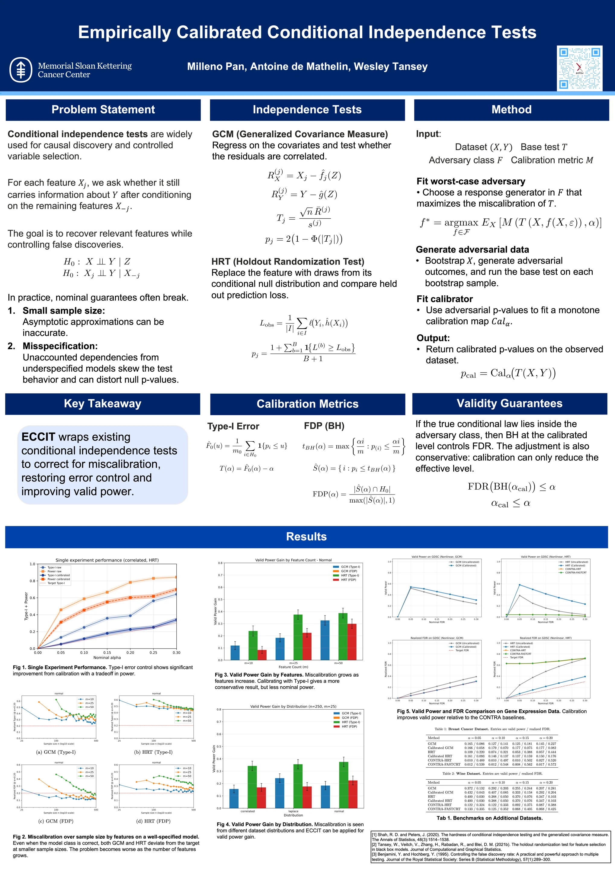
Empirically Calibrated Conditional Independence Tests

Milleno Pan, Antoine de Mathelin, Wesley Tansey

Empirically calibrated conditional independence testing (ECCIT) for false discovery rate control.

Summary

Conditional independence tests drive causal discovery and feature selection, but in practice they often break their error guarantees, even with false discovery rate (FDR) control. Small samples undermine asymptotic guarantees, and misspecified models skew p-values under the null. ECCIT measures and corrects this miscalibration. For a base test such as GCM or HRT, an adversary searches for the features and response functions that miscalibrate it most, and ECCIT then fits a monotone map that adjusts the test’s p-values to match. On synthetic and real data, it achieves valid FDR with higher power than existing calibration methods.

Method
  1. 01

    Fit a worst-case adversary

    Search a class of plausible responses for the one that breaks the test worst: which features matter (γ) and how (f).

  2. 02

    Generate adversarial data

    Resample rows of the real X and draw outcomes Ỹ from that adversary, so we know exactly which features are null.

  3. 03

    Measure the miscalibration

    Run the base test (GCM, HRT, …) on each resample. Its null p-values should be flat; the pile-up near zero is the error.

  4. 04

    Fit the calibrator

    Learn a monotone map from raw to calibrated p-values, then apply it to the test’s p-values on the real data.

Algorithm 1 in the paper
Calibration
Possible generators Worst case

The adversary tries many plausible ways the data could have been generated and keeps the one that makes the test fail worst. Calibrating against that worst case brings every one of them to or under the target. Simulation · GCM · n = 60, m = 25 · sparse linear responses, Gaussian / Laplace / t noise
False discoveries
Discovery False discovery Not selected Cut-off (BH, α = 0.2)

One simulated dataset where we know the answer. Taller stems are stronger evidence, and everything above the line is reported as a discovery. The raw test finds all 8 real signals but adds 4 false ones, so 4 of its 12 discoveries (33%) are false against a 20% target. After calibration it finds 7, none false. Simulation · GCM · n = 60, m = 25 · Benjamini–Hochberg at α = 0.2

Published in

Proceedings of the 29th International Conference on Artificial Intelligence and Statistics (AISTATS), PMLR 300:5194–5202, 2026


Research experience

02

Work

03

Education

04

Skills

Languages

  • Python
  • Java
  • Go
  • SQL
  • JavaScript
  • TypeScript
  • R
  • Julia
  • C
  • C++
  • Bash

Frameworks & Tools

  • PyTorch
  • JAX
  • TensorFlow (Keras)
  • Hugging Face
  • scikit-learn
  • NumPy
  • pandas
  • SciPy
  • React
  • Node.js
  • Docker
  • Kubernetes
  • Slurm
  • Linux

Cloud

  • Google Cloud
  • AWS (EC2, S3, Lambda, DynamoDB)